手撕 DiT
实现一个轻量级的 DiT (Diffusion Transformer) 架构,结合了目前前沿的 Flow Matching (流匹配) 范式,并在自定义的模拟数据集上完成了完整的训练与欧拉法采样闭环。
DiT 架构核心原理
DiT (Diffusion Transformer) 的核心思想非常简单粗暴但极其有效:用 Transformer 替换掉传统 Diffusion 模型(如 DDPM)中常用的 U-Net 架构。 它的成功证明了 Transformer 在视觉生成任务上同样具备强大的 Scaling Law。DiT 的架构主要依赖以下几个关键机制:
图像块化 (Patchify) :继承自 ViT 的思想。DiT 将输入的潜变量空间切分成不重叠的 Patch,并展平为一维序列,将图像生成转换为标准的序列建模任务。条件注入 (adaLN-Zero) :模型需要知道当前时间步 t t t y y y γ \gamma γ β \beta β α \alpha α 极简目标 (Flow Matching) :这套代码使用了 Flow Matching 而非 DDPM。它构建了一条从纯噪声 x 0 ∼ N ( 0 , I ) x_0 \sim \mathcal{N}(0, I) x 0 ∼ N ( 0 , I ) x 1 x_1 x 1 x t = x 0 + t ⋅ ( x 1 − x 0 ) x_t = x_0 + t \cdot (x_1 - x_0) x t = x 0 + t ⋅ ( x 1 − x 0 ) v = x 1 − x 0 v = x_1 - x_0 v = x 1 − x 0
环境准备与全局设置
这部分主要负责导入必要的库,并固定随机种子以保证实验的绝对可复现性。
1
2
3
4
5
6
7
8
9
10
11
12
13
14
15
16
17
18
19
import torchimport torch.nn as nnimport torch.nn.functional as Ffrom torch.utils.data import DataLoader, TensorDatasetimport matplotlib.pyplot as pltimport numpy as npimport os"images" , exist_ok=True )def set_seed (seed=42 ):True 42 )
时间位置编码
时间位置编码 (SinusoidalPositionEmbeddings)
作用 :将连续的时间步 t ∈ [ 0 , 1 ] t \in [0, 1] t ∈ [ 0 , 1 ]
1 2 3 4 5 6 7 8 9 10 11 12 13 14 15 16 17 class SinusoidalPositionEmbeddings (nn.Module):def __init__ (self, dim ):super ().__init__()self .dim = dimdef forward (self, time ):self .dim // 2 10000.0 )) / (half_dim - 1 )None ] * embeddings[None , :]1 )return embeddings
解读 :这是经典的 Transformer 位置编码公式实现。通过 sin 和 cos 的组合,它能将标量时间转化为具有周期性特征的 dim 维张量,这是后续生成 adaLN 调制参数的原始信号源。
核心机制:DiT Block 与 adaLN-Zero
作用 :DiT 的特征提取基石。包含了 Self-Attention、MLP 以及最核心的 6 参数 adaLN-Zero 调制层。
1 2 3 4 5 6 7 8 9 10 11 12 13 14 15 16 17 18 19 20 21 22 23 24 25 26 27 28 29 30 31 32 33 34 35 36 37 38 39 40 41 42 43 44 45 46 47 48 49 50 51 52 53 54 55 56 class DiTBlock (nn.Module):def __init__ (self, hidden_size, num_heads, mlp_ratio=4.0 ):super ().__init__()self .norm1 = nn.LayerNorm(hidden_size, elementwise_affine=False , eps=1e-6 )self .attn = nn.MultiheadAttention(hidden_size, num_heads, batch_first=True )self .norm2 = nn.LayerNorm(hidden_size, elementwise_affine=False , eps=1e-6 )int (hidden_size * mlp_ratio)self .mlp = nn.Sequential(self .adaLN_modulation = nn.Sequential(6 )self .adaLN_modulation[-1 ].weight)self .adaLN_modulation[-1 ].bias)def forward (self, x, t_emb ):self .adaLN_modulation(t_emb)6 , dim=-1 )None , :]None , :]None , :]None , :]None , :]None , :]self .norm1(x)1 + scale_mha) + shift_mha self .attn(x, x, x)self .norm2(x)1 + scale_mlp) + shift_mlp self .mlp(x)return x
解读 :这是全篇最精妙的地方。elementwise_affine=False 是必须的,因为规范化参数交给了 adaLN_modulation 接管。全 0 初始化意味着在训练的第一步,scale 和 shift 为 0(等价于普通 LayerNorm),gate 也为 0(等价于 x = residual + 0)。这让初始网络成了一个完美的恒等映射,梯度可以毫无阻碍地传导,极大地加速了早期收敛。
宏观架构:DiT 主干网络
作用 :处理图像到序列的转换 (Patchify),融合时间和类别条件,并利用堆叠的 DiT Blocks 提取特征,最终还原回图像维度。
1 2 3 4 5 6 7 8 9 10 11 12 13 14 15 16 17 18 19 20 21 22 23 24 25 26 27 28 29 30 31 32 33 34 35 36 37 38 39 40 41 42 43 44 45 46 47 48 49 50 51 52 53 54 55 56 57 58 59 60 61 62 63 64 65 66 67 68 69 70 71 72 73 74 75 76 77 78 79 80 81 82 83 84 85 86 87 88 class DiT (nn.Module):def __init__ ( self, input_size=32 , patch_size=2 , in_channels=4 , hidden_size=256 , depth=6 , num_heads=8 , mlp_ratio=4.0 , num_classes=4 ):super ().__init__()self .in_channels = in_channelsself .patch_size = patch_sizeself .num_patches = (input_size // patch_size) ** 2 self .patch_embed = nn.Conv2d(in_channels, hidden_size, kernel_size=patch_size, stride=patch_size)self .pos_embed = nn.Parameter(torch.zeros(1 , self .num_patches, hidden_size))self .time_embed = nn.Sequential(self .class_embed = nn.Embedding(num_classes, hidden_size)self .blocks = nn.ModuleList([for _ in range (depth)self .norm_final = nn.LayerNorm(hidden_size, elementwise_affine=False , eps=1e-6 )self .final_modulation = nn.Sequential(2 )self .head = nn.Linear(hidden_size, patch_size * patch_size * in_channels)self ._init_weights()def _init_weights (self ):self .pos_embed, std=0.02 )self .head.weight, std=0.02 )self .head.bias)self .final_modulation[-1 ].weight)self .final_modulation[-1 ].bias)def forward (self, x, t, y=None ):0 ]self .patch_embed(x)2 ).transpose(1 , 2 )self .pos_embedself .time_embed(t)if y is not None :self .class_embed(y)for block in self .blocks:self .final_modulation(t_emb).chunk(2 , dim=-1 )self .norm_final(x)1 + scale_final[:, None , :]) + shift_final[:, None , :]self .head(x)int (self .num_patches ** 0.5 )self .patch_size1 , 2 ).reshape(B, self .in_channels, p, p, h, w)'n c p q h w -> n c h p w q' , x)self .in_channels, h * p, w * p)return x
解读 :这里的重点在于特征空间的转换。输入是 [B, C, H, W],经过 patch_embed 变成了 [B, Seq_Len, Hidden],加上了位置编码 pos_embed 后进入 Blocks。在输出阶段,通过一个 Linear 层和 einops 风格的重排(einsum+reshape),将 Transformer 处理完的一维序列,完好无损地拼接回了原始的图像分辨率。
模拟数据集与 Flow Matching 损失函数
作用 :为了快速验证模型,使用 Numpy 生成了几何图案作为真实数据分布;利用 Flow Matching 构建从高斯噪声到数据的直线目标。
1
2
3
4
5
6
7
8
9
10
11
12
13
14
15
16
17
18
19
20
21
22
23
24
25
26
27
28
29
30
31
32
33
34
35
36
37
38
39
40
41
42
43
44
45
46
47
48
49
50
51
52
53
54
55
56
57
58
59
60
61
62
63
64
65
66
67
68
69
def generate_simulation_dataset ( num_samples=2000 , img_size=32 , in_channels=4 , num_classes=4 , noise_level=0.05 """ 生成带类别规律的模拟DiT训练数据集 """ for class_id in range (num_classes):for _ in range (samples_per_class):if class_id == 0 :2 * xx)elif class_id == 1 :4 * yy)elif class_id == 2 :3 * xx) * np.sin(3 * yy))else :2 + yy**2 ) / 2 ) * np.cos(4 * np.sqrt(xx**2 + yy**2 ))0.1 * i for i in range (in_channels)0 )0 , noise_level, multi_channel_pattern.shape)max (np.abs (multi_channel_pattern))return data, labelsdef flow_matching_loss (model, x1, y=None ):""" Flow Matching 核心损失 x1: 真实数据 y: 类别标签 """ 0 ]None , None , None ] return loss
解读 :flow_matching_loss 完美展现了当前主流(如 Stable Diffusion 3 都在用)的 Flow Matching 的优雅之处。相比 DDPM 复杂的 α t \alpha_t α t β t \beta_t β t x 1 x_1 x 1 x 0 x_0 x 0 x 1 − x 0 x_1 - x_0 x 1 − x 0
训练与推理采样 (Euler Method)
作用 :调度优化器进行模型训练,并通过常微分方程 (ODE) 的欧拉方法,根据预测的向量场逆向生成图像。
1
2
3
4
5
6
7
8
9
10
11
12
13
14
15
16
17
18
19
20
21
22
23
24
25
26
27
28
29
30
31
32
33
34
35
36
37
38
39
40
41
42
43
44
45
46
47
48
49
50
51
52
53
54
55
56
57
58
59
60
61
62
63
64
65
66
67
68
def train_dit (epochs=50 , batch_size=64 , lr=1e-4 , device=None ):if device is None :"cuda" if torch.cuda.is_available() else "cpu" )print (f"使用设备: {device} " )print ("正在生成模拟数据集..." )2000 )True , drop_last=True )1e-4 )1.0 sum (p.numel() for p in model.parameters())print (f"模型总参数量: {total_params / 1e6 :.2 f} M" )print ("开始训练..." )for epoch in range (epochs):0.0 for batch_x1, batch_y in dataloader:0 ]len (dataset)if (epoch + 1 ) % 5 == 0 :print (f"Epoch [{epoch+1 } /{epochs} ], 平均损失: {avg_loss:.6 f} , LR: {scheduler.get_last_lr()[0 ]:.6 f} " )print ("训练完成!" )return model, loss_history, data, labels@torch.no_grad() def dit_sample (model, num_samples=8 , class_id=0 , img_size=32 , in_channels=4 , num_steps=20 , device=None ):if device is None :"cuda" if torch.cuda.is_available() else "cpu" )eval ()1.0 / num_steps0 , 1 - dt, num_steps, device=device)for t in t_list:return x.cpu()
解读 :采样函数 dit_sample 实现了从纯噪声变回数据的魔法。由于 Flow Matching 的公式是 d x d t = v ( x , t ) \frac{dx}{dt} = v(x, t) d t d x = v ( x , t ) x = x + v_pred * dt 实现了最简单的数值积分(欧拉法),每一步都沿着模型指引的方向往前走一小步 dt,经过 20 步就能逼近真实的图像流形。
可视化与执行入口
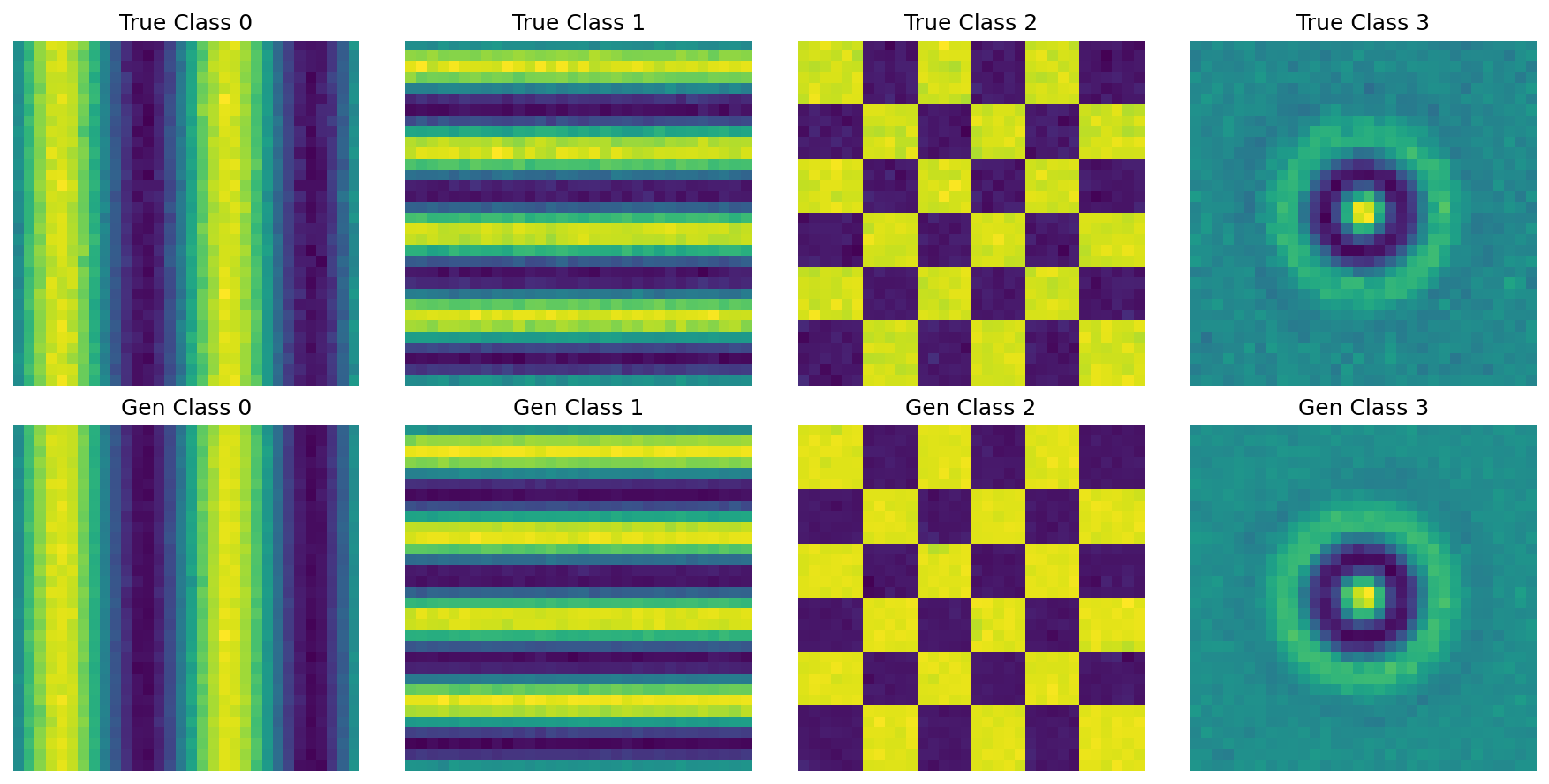
作用 :将训练结果直观展示,对比真实分布和生成的分布。
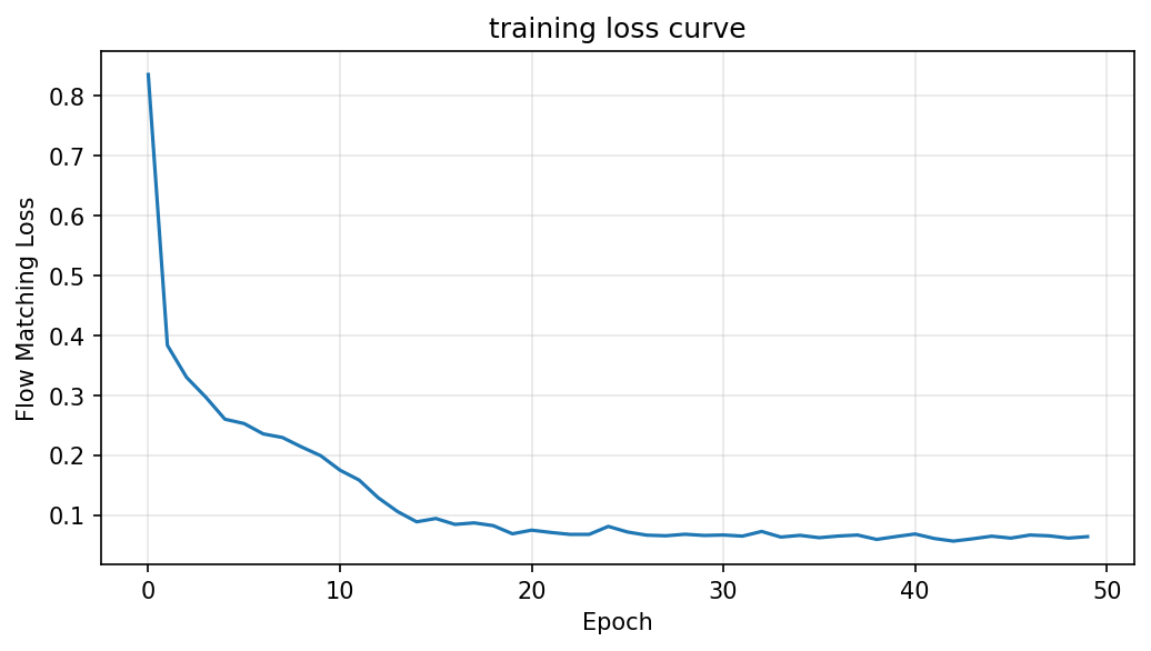
1 2 3 4 5 6 7 8 9 10 11 12 13 14 15 16 17 18 19 20 21 22 23 24 25 26 27 28 29 30 31 32 33 34 35 36 37 38 39 40 41 42 43 44 45 46 47 48 49 50 51 52 53 54 55 56 57 58 59 60 61 62 def visualize_all_classes (real_samples, gen_samples, num_classes=4 ):""" 对比可视化:所有类别的真实数据 vs 生成数据(放在同一张图) 第一行:真实图像,第二行:生成图像 """ 3 , 6 ))for cls_idx in range (num_classes):2 , num_classes, cls_idx + 1 )0 ], cmap='viridis' )f"True Class {cls_idx} " )'off' )2 , num_classes, cls_idx + 1 + num_classes)0 ], cmap='viridis' )f"Gen Class {cls_idx} " )'off' )"images/all_classes_comparison.png" , dpi=150 , bbox_inches='tight' )def plot_loss_curve (loss_history ):8 , 4 ))"training loss curve" )"Epoch" )"Flow Matching Loss" )True , alpha=0.3 )"images/loss_curve.png" , dpi=150 , bbox_inches='tight' )if __name__ == "__main__" :50 )0 , 1 , 2 , 3 ]print ("\n正在生成所有类别的样本..." )for cls in target_classes:0 ]1 , class_id=cls)0 ])print ("\n所有任务完成!生成的图片已保存到 images 文件夹" )
训练损失和真实图像和生成图像展示